Does temperature influence where an animal wants to live? How do we find out?
Developed by Dhruba Naug, Sarah Jaumann, Chris Mayack and Ryan Joyal
This is a relatively simple and straightforward biology experiment intended as a lesson plan to introduce upper elementary-level students to the scientific method, using the context of animal behavior and ecology. Teachers can also use this template as a tool to develop their own experiments for other topics. When used as an introduction to animal behavior and ecology, students really enjoyed and had fun with this activity! Specifically, they measured and compared the temperature preferences of different insects using a thermal gradient and used this information to predict the habitat preference of each insect. Although the main focus of the activity is the exposure to the methods of scientific experimentation, mathematical concepts such as calibration curves, graphing, and summary statistics are also incorporated. The whole experiment should ideally be spaced over two consecutive days.
Ideal grades: 4-6; 7- 8 with modification
Optimal class size: 18- 24 students
Optimal group size: 3- 6 students
Time needed for activity: Two consecutive days: 1 to 1¼ hours on Day 1, 1½ to 2 hours on Day 2
Preparation time: 2 hours to construct the gradient, 2 hours to calibrate it, 5 minutes of set-up before activity (but should be done 1 ½ hours beforehand)
Curriculum that best accommodates activity: ecology and life zones/ habitats, scientific method
Budget: $25-40 (assuming that gradients can be made in-house)
Materials: 1) Two different types of insects. Crickets and bark beetles are good choices. Field crickets have a relatively high temperature preference (~ 40- 50°C), while certain darkling beetles have lower preferences (~25- 35°C). Crickets can be purchased at pet stores (the large size works best because they are easier to spot). The species of beetle used in this experiment was from the Tenebrionidae family and are commonly known as skunk beetles. These can be collected by the hundreds after summer rains from the high plains steppe of eastern Colorado, for example on the Pawnee National Grassland. Alternatively, superworms can be purchased from pet stores and maintained until adulthood for the purpose of this experiment. They are in the same family as the skunk beetles.
2) Vials for holding the insects.
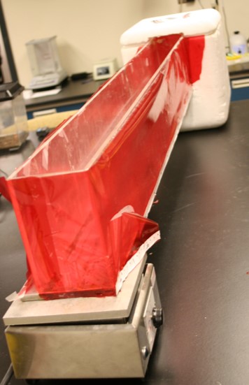
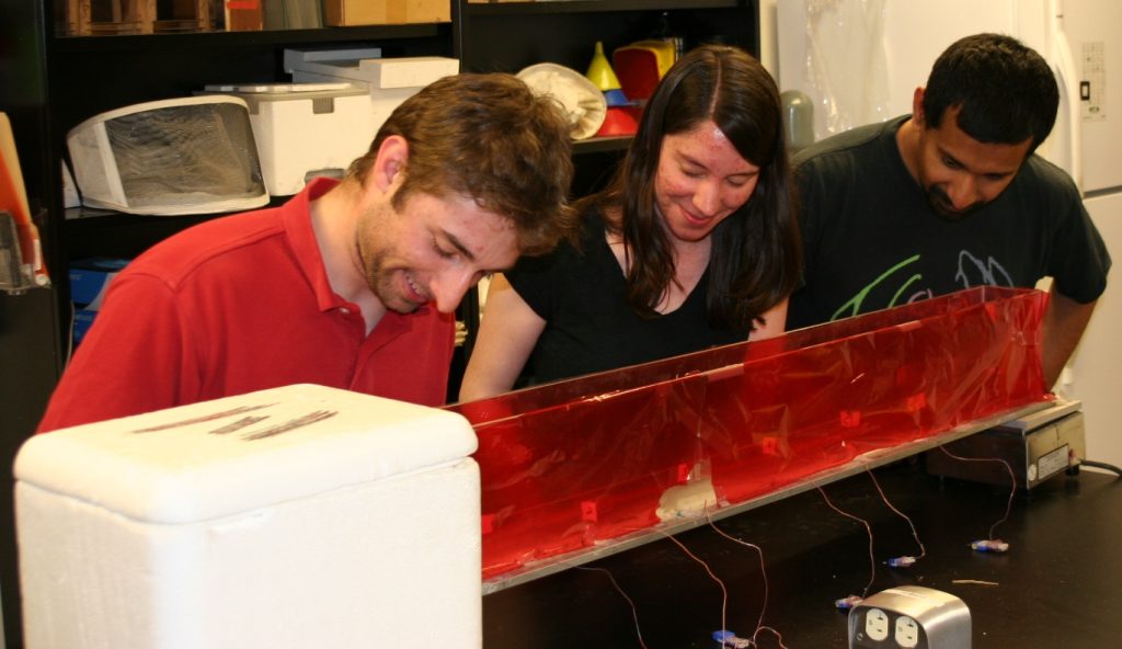
3) Thermal gradients. The number of gradients needed depends on the number of students participating. Six or fewer students per gradient is ideal; more than six becomes a bit chaotic. We worked with about 24 students, three gradients, and three adult leaders (click here to view instructions for the construction of a thermal gradient).
4) Hot plates and Styrofoam ice chests – one each per gradient.
5) Crushed ice (cubes don’t cool the gradient as well).
6) One digital thermometer per gradient.
7) Pictures of insects (optional).
8) Each student needs a pencil and experiment packet (click here to see an example of a packet).
Pre-Experimental Preparation:
1. Construction of thermal gradients.
2. Calibration of thermal gradients – Fill the Styrofoam box with crushed ice and turn on the hot plate and adjust its temperature to about 125°C. It takes a bit of trial and error to figure out how high to set the hot plates for each gradient. Each hot plate, gradient, and ice chest will probably be different, so it is a good idea to keep them as sets and calibrate them separately. Make sure that the gradient end with the lower numbers is inserted into the ice chest while the end with the higher numbers rests on the hot plate so that the students see a positive correlation between distance and temperature. While a graph with a negative slope of course does not matter for calibration purposes, in our experience we found that the children had a little trouble making the connection in such a case. Also make sure that the temperature range to which the gradient is set corresponds to the scale of the graph drawn in their exercise packets.
3. Obtain insects and perform a trial run. If beetles are used, they should be relatively large as small beetles sometimes turn upside down and are not able to right themselves, which results in their immobility (although this can give someone an idea for a different experiment, it is not conducive to the success of this particular experiment).
Day 1- Introduction, Hypotheses, and Calibration Curves: Set up the gradients 1 ½ hours before the exercise to let them reach an equilibrium temperature. Allow 1 to 1¼ hours.1. Introduction – We introduced the experiment to the kids by giving a brief, general explanation of what it was about and what they were going to do (and how much fun it was going to be!). Key question: Why is it important to do an experiment in order to make a scientific inquiry instead of just observing what happens in nature?We did this experiment following a study of life zones the students do as a part of their regular curriculum. So we introduced the experiment with the question that if they observed different insects in different life zones, does that necessarily mean the insects inhabit those zones and if there is a way to test it. We then gave a brief background about what an insect is (this was where pictures come in handy), and refreshed their memory of where one might find crickets and the beetles.
2. Questions to be tested- Which insect will prefer a higher temperature and why? What these temperatures are likely to be? What might this say about their preferred habitat and life zone?
3. Calibration Curves- We pointed out that it is usually difficult to measure the value of a dependent variable at every possible value of the independent variable that determines it and one uses a standard curve to deal with this issue. For example, in this experiment it is not feasible to directly measure the temperature at every single point on the gradient. Use some other examples to clarify this concept. The students were then divided into three groups of six each and allowed to measure the temperature with the digital thermometer at six distances. They plotted these measurements on the graph in their exercise packet and drew a best-fit line representing all the points. Using the numerical exercises in the packet, we then made the students familiar with using the calibration curve.
Day 2- Experiment, Results, and Conclusion: Allow 1½ to 2 hours. Crickets were put into vials before arrival at the school so that it is easy to introduce them into the gradient.
1. Experiment- After a brief reminder of where we were in the experiment the previous day, the students broke into the SAME groups as the previous day so that they could use the same calibration curves they constructed. The students in each group were divided between the two lanes in the gradient. The insects were then introduced into the gradient and the experiment began. Students took recordings of only one insect – the one in the lane they were assigned to. The position of the insect was recorded in cm every minute for 15 minutes by one student and this distance was translated into a temperature using the calibration curve by a second student. We let students interchange their roles during the experiment so that everyone could experience everything. One of the adults kept track of the clock and shouted out the minutes so that all the students could make the recordings at the designated intervals.
**NOTE: It is a good idea to write down all the recordings in a single exercise packet during the experiment and then have everyone copy them down at the end of the experiment. This avoids confusion and works faster.
2. Results – At the end of the experiment, after each student had copied the data on both the insects in their gradient, they were allowed to calculate the minimum, maximum, median, mode, range, and mean temperature observed for each insect. The students then made a line graph for each insect that showed the change in temperature preference with time over the duration of 15 minutes.
**NOTE: For calculating the averages, it is a good idea to break up the set of 15 numbers for each insect into sets of 5 because it is easier for them to add five numbers rather than 15. Once you have the sums for each of the three sets, they can add those three numbers and divide it by 15 to get the average.
3. Conclusion – We asked the students whether the data they collected matched their initial hypotheses about the temperature preference of the insects. If the data did not match their hypotheses, we encouraged them to come up with reasons that could have led to the observed result. We also compared data across the different groups and gave them some idea about the value of replicates while doing an experiment, variability etc. We also tried to spend some time discussing the possible experiments that could be developed in the future based on what we learned here.